Benchmark Dose Software (BMDS) is often used to set “safe exposure” limits, which serve as the basis of regulations for safe levels of chemicals. These limits must be derived correctly; if they are set too high, public health may be at risk; if set too low, millions or billions of dollars will be spent unnecessarily reducing chemicals to levels that do not pose a public health risk. The EPA uses BMDS modeling in its chemical risk assessments to support guidance and regulations.
Dr. Shao [1] felt obligated to promote scientific integrity and alert the scientific community to the problems with the current version of EPA’s BMDS modeling. Most people who use BMDS modeling are non-statisticians and won’t understand the methodological flaws. According to Dr. Shao, if EPA uses this modeling approach to support its policy,
“the scientific rigorousness and the integrity of those risk assessments [which will support policy making later] will be compromised.”
BMD modeling
When EPA sets regulations, it needs to consider the effects of a chemical on a person’s health after exposure to it in the environment, primarily from breathing air or drinking water. EPA uses different models to set regulations for chemicals in the environment. [2] Because it is not possible to directly determine the amount (dose) of the chemical that may be affecting people after long-term exposure, EPA often uses studies in laboratory animals to do this.
BMD modeling is used because it considers the effects of chemicals on human health at very low levels in the environment using the results from studies in laboratory animals [3] to estimate the dose of a chemical that will cause a biological response. It was first developed in the 1980s and adopted by EPA in the mid-1990s for risk assessment. It may be considered an elaborate form of regression analysis, a statistical technique used to explore the relationship between two or more variables.
BMD modeling only considers how much of a chemical results in a biological response and does NOT consider factors such as how many people are exposed to a chemical, where exposure occurs, or the likelihood of exposure. There are other models and methods used to factor those considerations.
The graph below shows the results from an animal experiment and the terms used to describe the results in BMD modeling.
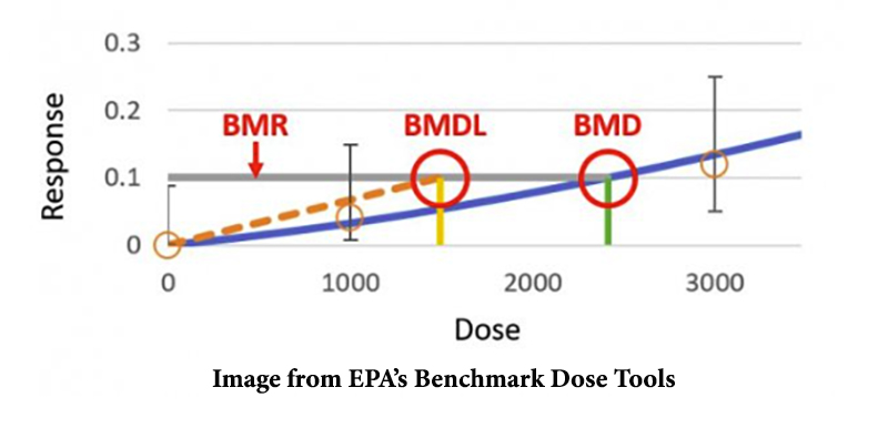
- BMR (benchmark response): the predetermined change in biological response (usually 5% – 10% change in response rate). Responses commonly modeled are body weight, cell proliferation, red blood cell count, tumor incidence rate, and percentage of animals developing an adverse effect.
- BMDL: lower confidence level of the BMD.
- BMD (benchmark dose): a chemical dose that produces a predetermined change in an adverse effect, such as weight loss or tumor incidence.
The statistical lower bound of a benchmark dose (BMD) is the most crucial term because this is the level often used by EPA to derive the “safe exposure” level in its regulations. If this level is not modeled correctly, the entire regulation could be determined to be based on inadequate science and thrown out by the courts in litigation.
For modeling purposes, responses are divided into two types:
- Dichotomous response: presence or absence of an effect, e.g., the presence or absence of a tumor.
- Continuous response: an actual measurement or a relative change from control, e.g., percent increase in body weight compared to controls.
This is critical because classifying the type of responses plays a significant role in the shortcomings of EPA’s modeling function.
Benchmark Dose Software (BMDS)
In 2000, the EPA first released their BMDS as standalone software. In 2017, the EPA released the last version of the standalone BMDS, using a frequentist method, looking at the data to determine the maximum likelihood estimation (MLE). For example, if it rained 8 out of 10 days in the past on similar days, we might estimate the chance of rain to be 80%.
In 2018, the EPA released its first Excel-based BMDS, adding the “Bayesian” modeling function, which looks at data and other useful information. The Bayesian method takes useful information, termed a prior distribution, and updates probability as new or more data become available. The updated probability is termed the posterior probability.
To understand the difference, consider the classic problem of “Let’s Make a Deal.” You are faced with three doors. Behind two of the doors, there are goats, and behind one door, there's a car. You pick a door, and the host (who knows what's behind each door) opens one of the other two doors to reveal a goat. Do you stick with your original choice or change your mind?
Frequentist Analysis:
Before any doors open, each door has an equal probability of 1/3 of hiding the car. When the host opens a door to reveal a goat, the frequentist approach doesn't change the initial probabilities. Your chosen door still has a 1/3 chance of hiding the car. According to frequentist analysis, the probabilities for each door remain the same after the host opens a door. The fact that you now know the location of one goat doesn't affect these probabilities.
In the frequentist view, there is no advantage to switching or sticking, and each door retains its original probability.
Bayesian Analysis:
Before any doors open, the probability of the car being behind your chosen door is 1/3, and the probability of the car being behind one of the other doors is 2/3. When the host opens a door to reveal a goat, the probabilities don't change for your chosen door (1/3 chance of having the car) because your choice was made before any doors were opened. However, the probability for the unopened door increases to 2/3 because the car must be behind either your original choice or the other unopened door. The Bayesian approach says you should switch because the probability of the car being behind the other unopened door is now higher compared to sticking with your initial choice (1/3). The Bayesian strategy, therefore, suggests always switching to maximize your chances of winning the car.
In the world of Bayesian probability, the strategy is to stay flexible, adapt to new information, and maximize your chances of success based on the most recent data.
Errors According to Dr. Shao
In the new BMDS, EPA added the “Bayesian” modeling function for continuous and dichotomous data (and promptly removed it for continuous data). But this modeling function is not a true Bayesian analysis; instead, it uses a “Laplace approximation,” which can approximate a full Bayesian analysis under special circumstances. But Laplace’s approximation is valid and works well only for large sample sizes. Because of this, Laplace’s approximation does not work well for typical dose-response modeling and BMDS estimation in risk assessment, which has a small sample size.
Additionally, with a small sample size, the prior distribution becomes increasingly important; small changes can create significant differences in outcome; it must have a firm scientific basis. This was not the case with the prior distribution selected by EPA for use in the “Bayesian” modeling function. The only advantage of Laplace’s approximation method over the full Bayesian analysis is that it is more computationally efficient, requiring a shorter processing time.
Other problems with the “Bayesian” modeling function implemented in BMDS include:
- It was tested only on datasets with large sample sizes; the limitations on datasets with small sample sizes, typically used in BMDS modeling, were not exposed.
- EPA ignored important factors of model fit, such as goodness-of-fit and model weight, and focused only on model-averaged BMD estimates.
- No information was given on how the critical prior distributions used in BMDS were derived, merely stating “by design.” Many of these prior distributions were altered with no justification provided or peer review conducted.
EPA removed the “Bayesian” model for continuous data but left the model for dichotomous data, probably because the mistakes in dichotomous data are not as apparent as in continuous data. Each of the problems individually is problematic; taken together, the result is a model that produces flawed results.
Dr. Shao urged EPA to conduct a comprehensive and unbiased investigation of the “Bayesian” model in BMDS, but they did not do that. Instead, they have not only included this approach in BMDS, but they have also made it the default and only choice for modeling dichotomous data. Dr. Shao strongly urges the EPA to remove this approach until they can justify its plausibility and scientific rigor. Since this model is used as the basis of so many EPA regulations, it is critical that it is correct.
A sincere thank you to Dr. Shao for taking the time from his busy schedule to answer questions about technical statistical issues to a non-statistician.
[1] Dr. Shao is an expert in chemical risk assessment and runs the Computational Risk Assessment Laboratory at Indiana University School of Public Health. He has a dual Ph.D. in Civil and Environmental Engineering and Engineering and Public Policy. He has been widely published in his field of expertise: “developing innovative and computational approaches to advance dose-response analysis (especially benchmark dose modeling) to support chemical risk assessment.”
[2] Examples include trichloroethylene, benzene, perfluorooctanoic acid (PFOA), mercury, and chromium.
[3] Studies in humans can also be used in BMD modeling, but this is rarely done due to the lack of available studies that meet the modeling requirements.