
Air pollution epidemiology has tended to emphasize premature mortality; the NIH database lists over 3000 papers with those terms in the title or abstract. But no specific causes of death are uniquely linked to air pollution; studies have focused on non-accidental, cardio-respiratory, and cancer deaths. Fatalities reported in these studies are rare, typically < 0.5% of the population [1], implying that victims are not selected randomly but may comprise the frailest subjects having the most significant exposures. By and large, in the U.S., these studies have been designed to support regulatory interests under the Clean Air Act rather than scientific inquiry. EPA selects the pollutants of concern, the locations to be monitored (outdoors), and the timeframes of interest. Locations range from zip-codes to regions and may focus on presumed “hot-spots” rather than population centers. Frequencies of monitoring may be limited by air sampling technology, duration limited by the study’s arbitrary timeframe. Many recent studies have been focused on single pollutants of particular regulatory interest. These parameters define the feasible space-time regions for epidemiological research. The onset and timing of air pollution-related premature mortality garner less attention than geography per se.
The space-time “pie” and epidemiological methods
Picture an inverted deep-dish pie as a space-time region with the spatial (geographic) domain as the horizontal axis and the temporal dimension as vertical. Cross-sectional (XS) analysis slices the pie horizontally, i.e., spatially, and the thickness of the slice defines the time domain, from days to years. Longitudinal or time-series studies (TS) slice the pie vertically, over time, the widths of those slices define spatial domains, usually one or more metropolitan areas. Neither technique samples the entire pie. The width of a slice determines the observable detail irrespective of how the pie is sliced. TS study analyzes how mortality rates vary over time within selected spaces whose populations may differ in terms of underlying susceptibilities. XS study analyzes spatial variability for a given time period during which all variables may have undergone important temporal trends that must also be considered, especially disease latency and cumulative exposures.
The existing literature tends to be formulaic, using well-established regression methods and data that vary by location, period, pollutant, cause of death. Studies tend to focus on achieving a specified degree of precision (statistical significance) that is dependent on sample size. Just as correlation does not infer causality, statistical significance does not imply physiological significance or a plausible time frame. The long-term causality of mortality associations has not been demonstrated.
The level of detail, the granularity within a “slice,” defines the precision of the analysis; studying zip-codes can be more informative than studying entire states, and daily analyses are more informative than annual, within data availability. Critical hazards like heavy smoking or traffic density are often unevenly distributed geographically, and averaging across a metropolitan spatial domain obscures details of the individual residences that define personal exposures.
The importance of timing
Health outcomes are time-dependent; the incidence of cancer and the ill-effects of smoking involve cumulative exposures over time, while cardiovascular events may be sensitive to daily peaks, for which duration can be important as seen in heatwaves. Acute responses may lag behind peak exposures by up to a week, for which the proper response metric is the sum over the lag period. Timing per se is rarely considered in air pollution epidemiology.
Questions have been raised about the prior health status of those who respond to short-term peak exposures. The importance of pre-existing conditions has been shown in epidemics like the current COVID-19. Healthy subjects are not at risk; excess mortality of the most susceptible (frail) subjects in a closed cohort is likely to be followed by reduced mortality among the surviving members. This “harvesting” hypothesis has been seen in conjunction with influenza epidemics but has not been observed in air pollution time-series analyses. In a dynamic population, increased frailty precedes susceptibility1 and provides newly frail subjects that are subsequently subjected to acute environmental exposures. Susceptibility may be associated with previous longer-term air pollution exposures.
Dose-response relationships
This space-time “pie” model offers two approaches for estimating pollution’s dose - mortality relationships: cross-sectional (XS) geographic analysis over a given time frame (492 NIH citations of long-term effects), or temporal analysis (TS) for a given region (885 NIH citations of daily analyses). Only 9% of the studies used both terms. Here I use simple graphical examples to illustrate how the two modalities should be analyzed jointly.
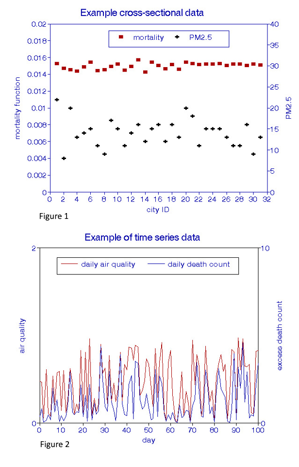
Examples of types of raw data are shown in Figures 1 and 2. XS data (Figure 1) are grouped by location (“city ID”), usually based on the availability of ambient air quality data throughout the period of interest. The stability of such relationships may be examined by considering other periods or groups of cities. The time-series data (Figure 2) are analyzed daily at a given location and could be replicated at different locations during the period of interest.
Dose-response relationships (deaths per unit of pollution) are derived from cross-plots. A valid XS analysis (Figure 3) must control for age, race, and gender and many other factors affecting the health status of residents, notably smoking habits, income, and obesity, as well as indoor exposures. 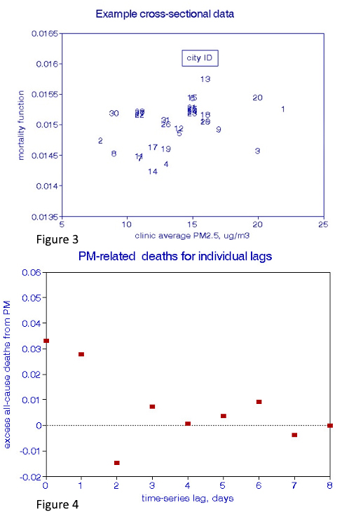 The ability to accomplish these requirements may be problematic, resulting in relatively wide confidence intervals (CIs). The observation period may be expanded to reduce confidence limits, but may simultaneously increase the temporal instability of the confounding variables.
Temporal studies of pollution’s dose-response (Figure 4) compare the correspondence between coincident mortality and pollution peaks and valleys after specified lag periods. Just as in XS studies, confounding temporal factors must be considered: daily weather, especially temperature, seasonal cycles, days of the week, holidays. Various methods have been devised to accomplish these requirements, but they all suffer from arbitrary decisions about how much seasonal control may be appropriate. Most of these studies searched for the lag interval yielding the most robust pairwise relationships; only a few considered lag intervals longer than two days, and even fewer examined cumulative effects during the lag period.
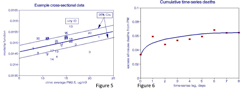
I added information to Figures 5 and 6 to further define the dose-response relationships. A regression line and its 95% CIs are added to the XS plot (Figure 5), while a curve-fitting line is drawn through the cumulative TS effects (Figure 6).
Finally, I superimposed these two plots in Figures 7 and 8 to compare the XS and TS relationships and the PM and O3 results.
Interpretation
The time-dependent process may be illustrated by considering a heterogeneous population along a time axis where corresponding peaks and valleys in air pollution and death counts are noted. The initial underlying health status and susceptible sub-populations most at risk may be associated with prior long-term exposures to various substances and other risk factors. When a peak air pollution exposure is encountered along the vertical ”slice,” some of the most susceptible members of the sub-population at risk may expire; those excess deaths are labeled as “pollution-related”. Over time, when another peak episode occurs, and additional newly susceptible members expire, those deaths are added to the pollution-related group. By the end of the period of study, the content of the pollution-related mortality group comprises the total short-term response to air pollution over the entire period. Their dose-response function is given by the ratios of excess deaths to excess pollution as determined by TS analysis and, as shown in Figure 6, summed over the lag period. This process should be repeated in other locations (i.e., slices) over the shared study period.
Those locations will vary in terms of overall average mortality rates, age, air pollution exposures, climate, personal risk factors like age, smoking habits, income, and underlying health. XS regression analysis is used to estimate the long-term dose-response relationship between average mortality rates and average pollution exposures across a group of locations (horizontal slice) controlling for the other variables and disease latency. Cumulative rather than coincident exposures are appropriate for some pollutants.
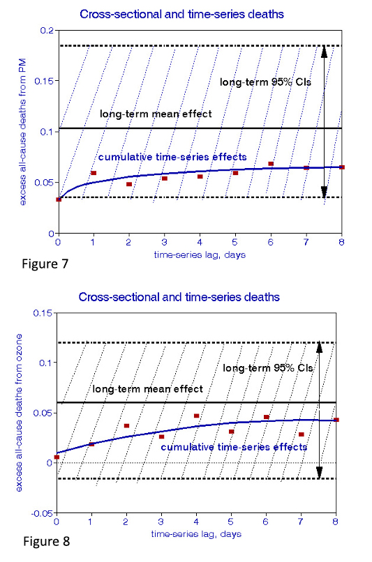 The XS relationships comprise all the time-dependent effects that occurred during the period of study, including the day-to-day relationships, and thus remain constant during the time interval, as indicated by the horizontal lines in Figures 7 and 8. The TS relationships are daily, aggregated over some arbitrary interval. The differences between XS and TS dose-response relationships demonstrate effects less frequent than daily, e.g., monthly as well as persistent effects of exposures before the period of study. Any true long-term effect could only be associated with differences between the XS and TS estimates. Given the typically wide CIs of dose-response relationships, these differences must be subjected to statistical significance testing. Figures 7 and 8 show that the differences are not significant in these examples, leading to the conclusion that daily effects dominate. As a result, the XS relationship in Figure 5 cannot be presumed to have caused new cases of chronic disease.
This finding does not preclude other associations with ambient air pollution in the long-term; the statistical significance of a cross-sectional relationship may indicate that some cities are more likely to experience short-term effects than others. This could be due either to sharper peak concentrations, more significant fractions of susceptible individuals, or the city’s prior pollution impacts. The relationship between air pollution and the onset of frailty has not been thoroughly investigated but clearly should be.
Conclusions
I have presented a framework for air pollution epidemiology that clearly discriminates between acute and chronic effects; no such studies have yet been published. I conclude that among the NIH-listed studies, short-term risks have been underestimated through failure to sum over sufficiently long lags. In contrast, long-term risks have been overstated by neglecting prior exposures and disease latency. I can find no credible evidence that air pollution induces new cases of chronic disease, conclusions that rest on issues of timing. Prior epidemiologic studies purporting to demonstrate that XS causes fatal chronic diseases are thus problematic. Time marches on, but our understanding of long-term air pollution health effects has not. Further air pollution health research should be directed towards processes that may induce susceptibility and frailty and to more comprehensive TS studies.
[1] Typical mortality studies may involve 50,000 – 100,000 deaths over a decade or more.
Reference
1. A new time-series methodology for estimating relationships between elderly frailty, remaining life expectancy, and ambient air quality. Inhal Toxicol. DOI: 10.3109/08958378.2011.638947